New version 3.2 of TMS Analytics & Physics library introduced FNC components for creating math applications with minimal code writing. The previous article described how to implement curve fitting. In this article, we’ll continue the theme and explain some advanced features for function approximation.

Generally, we use some standard basis functions for curve fitting: Fourier basis (sine and cosine functions), polynomials, exponent functions, and so on. In rare cases, we need specific basis functions to approximate the data. The TMS FNC math components provide a straightforward way to create a basis with any set of functions. Moreover, we can develop and test the basis right in design time.

The component for creating a basis with a set of user-defined functions is TFNCLinearBasis1D. The component provides the following published properties:

• Variable (TVariableProperty) – provides the name of the variable for the basis functions.
• Coefficient (TVariableProperty) – provides the name of the coefficient for the fitting problem.
• Order (integer) – number of basis functions for approximation (read-only).
• Expression (string) – math expression of the constructed function (read-only).
• Parameters (TParameterCollection) – a set of parameters for parametric basis functions.
• Functions (TParameterCollection) – a set of functions to construct the basis.

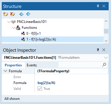
The two last properties provide the functionality to construct an arbitrary basis. With the Parameters property, you can add named values into the math environment and then use them to parametrize the set of basis functions. The Functions property allows to add, edit, and delete functions via standard Delphi collection editors. The collection contains items of TFormulaProperty type. When you add an item to the collection you can edit it with the Object Inspector as shown in the picture below. 

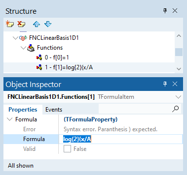
The class TFormulaPropery has several properties and a built-in mechanism to check the function for correctness. If you input a math expression that is not valid in the current context, the Error property will indicate what is wrong in the formula. An example is shown in the following picture.

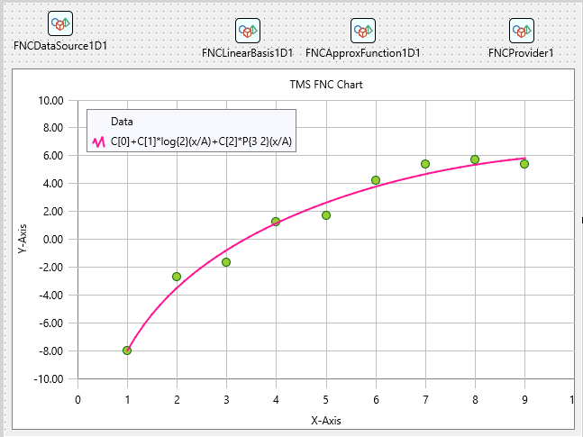
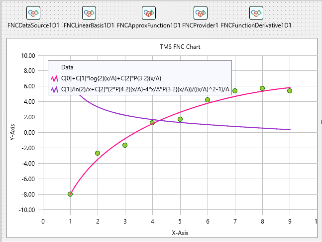
For our example, we created the collection with three basis functions: ‘1’, ‘log{2}(x/A)’ (logarithm to the base 2), and ‘P{3 2}(x/A)’ (associated Legendre polynomial of 3-rd degree and 2-nd order). Then, following the instructions described in the previous article, we added a data source, an approximated function, and a plotter to draw the function on the FNC chart. The final resulting FMX form at design time is shown in the picture below.

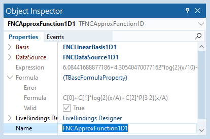
The main advantage of using the FNC math components is that you can select appropriate basis functions without running the application. At design time you can change parameter values and math expressions of basis functions. The changes will immediately affect the approximated function and you can see as the fitted curve looks on the FNC chart. Also, you can verify that the approximation succeeded by looking at the properties of the approximated function, as shown in the following picture.

Another feature of the FNC math components is that they work with symbolic data representation. Although the approximation uses discrete data as input, the result is a symbolic expression of the curve. So, we can use this expression for some advanced analysis. For example, we can evaluate the derivative of the function.

     The TFNCApproxFunction1D is a descendant of the TFNCBaseFunction1D class. Thus, we can use the same approach, as described in this article, to evaluate and draw the derivative of the fitted curve. The resulting designed form is shown in the picture below.

Note that the derivative is not evaluated numerically, as a finite difference for example. It is an analytical math function. So, this function can be evaluated at any point, not only at discrete points in the data source. Moreover, we can evaluate the fitted curve and its derivative at the points outside the data interval (for example, to predict how it is changed at the next point).

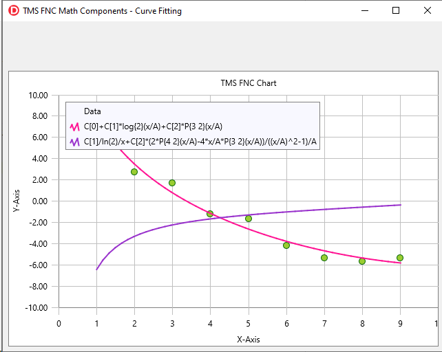
It is also easy to manage the parameters of approximation and other options at run time. For example, with the following small piece of code, we can update the data source.

var
  x, y: TArray<real>;
begin
  x:= [ 1.0, 2.0, 3.0, 4.0, 5.0, 6.0, 7.0, 8.0,
9.0 ];
  y:= [ 8.0, 2.7,
1.7,-1.2,-1.7,-4.2,-5.4,-5.7,-5.4 ];
  FNCDataSource1D1.AssignArray(x, y);
end;

When the data is assigned, the components are automatically updated and we can see the resulting fitted curve and its derivative on the chart.

The source code of the demo project for the article can be downloaded from here. You can install the TMS Analytics & Physics and TMS FNC Chart products and use many other useful features of the FNC math components.

Note that for students and teachers, there is also the free academic version of TMS Analytics & Physics. You can register for it from TMS Web Academy.