Blog
All Blog Posts | Next Post | Previous Post

 A simple computer algebra system with TMS Analytics & Physics 3.4
Monday, April 11, 2022
The main new feature of TMS Analytics & Physics 3.4 is the ‘Run’ method. This method is intended to execute commands, containing symbolic expressions.
Here is the code of a Delphi console application, that simulates a simple computer algebra system using the ‘Run’ method:
program Simulator;
{$APPTYPE CONSOLE}
{$R *.res}
uses
System.SysUtils,
Analytix.Utilities,
Analytix.Assembly,
Analytix.Float.Assembly,
Analytix.LinearAlgebra.Assembly,
Analytix.Derivatives.Assembly,
Analytix.Integrals.Assembly,
Analytix.Translator;
var
translator: TTranslator;
command, msg: string;
lines: TArray<string>;
i: integer;
begin
translator:= TTranslator.Create;
while true do
begin
Write('Input command: ');
ReadLn(command);
if command='' then exit;
translator.Run(command, msg);
lines:= msg.Split([#13]);
for i:=Low(lines) to High(lines) do
WriteLn(lines[i]);
WriteLn;
end;
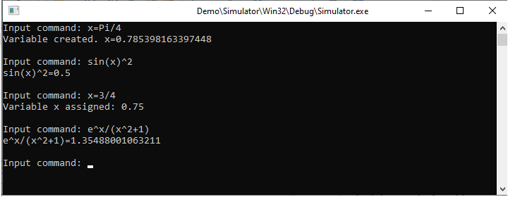
end.In the simplest case, we can use commands for creating new variables, assigning new values to the existing variables, or evaluating symbolic expressions, as shown in the picture below.
Assignment statement in the ‘Run’ method supports arrays, indexed expressions, and array slicing. Let us consider the following commands and the console output:
Input command: A=[1 -1 2 3/4]
Variable created. A=Array<Float>[4]=
(1 -1 2 0.75 )
Input command: B=[e 1/2 3 -3/4]
Variable created. B=Array<Float>[4]=
(2.71828182845905 0.5 3 -0.75 )
Input command: M=Matrix{3 4}(0)
Variable created. M=Array<Array<Float>>[3][4]=
( 0 0 0 0)
( 0 0 0 0)
( 0 0 0 0)
Input command: M[0]=A+B
Variable M[0] assigned: Array<Float>[4]=
(3.71828182845905 -0.5 5 0 )
Input command: M[2]=A-B
Variable M[2] assigned: Array<Float>[4]=
(-1.71828182845905 -1.5 -1 1.5 )
Input command: M
M=Array<Array<Float>>[3][4]=
(  3.71828182845905 -0.5  5   0)
(                 0    0  0   0)
( -1.71828182845905 -1.5 -1 1.5)
First, two arrays ‘A’ and ‘B’ are created, using so called array expression syntax (array elements in the brackets ‘[]’), and the ‘M’ matrix 3x4, using the ‘Matrix’ function. Then we assigned the sum of the arrays to the zero row of the matrix, and the difference of the arrays to the 2nd row. The assignment statement used so called array slicing feature. That is, we can use not entire matrix or its individual element, but also the part of the matrix – a row or a column. The library supports array expressions and slicing for Real, Complex, and Boolean arrays up to the 3 dimensions.
Another application of the assignment statement is creating user-defined functions. In the following example, we created two functions: the first calculates the volume of a sphere of radius ‘r’; the second calculates the length of a 3D vector, defined by the ‘x’, ‘y’, and ‘z’ coordinates.
Input command: V(r)=4/3*Pi*r^3
Function created. V(r)->4/3*Pi*r^3
Input command: L(x y z)=(x^2+y^2+z^2)^(1/2)
Function created. L(x y z)->(x^2+y^2+z^2)^(1/2)
Once a function is defined, it can be then used in expressions to calculate their values for the specified arguments:
Input command: V(1/2)
V(1/2)=0.523598775598299
Input command: L(-1 e 3/4)
L(-1 e 3/4)=2.99191512228048
The ‘Run’ method also supports more complicated commands, such as conditional statement and loop statement. The following console output shows how the user solves a square equation with specified coefficients ‘a’, ‘b’, ‘c’, using the conditional ‘IF’ statement:
Input command: a=1
Variable created. a=1
Input command: b=-2
Variable created. b=-2
Input command: c=-3
Variable created. c=-3
Input command: d=b^2-4*a*c
Variable created. d=16
Input command: IF{d<0}(NULL x1=(-b+d^(1/2))/(2*a))
IF: d<0=False, running x1=(-b+d^(1/2))/(2*a).
Variable created. x1=3
Input command: IF{d<0}(NULL x2=(-b-d^(1/2))/(2*a))
IF: d<0=False, running x2=(-b-d^(1/2))/(2*a).
Variable created. x2=-1
In the next example, the user calculates the sum of first 100 integer numbers, using the ‘FOR’ loop statement:
Input command: S=0
Variable created. S=0
Input command: FOR{i=1:100}(S=S+i)
i=1: Variable S assigned: 1
...
i=100: Variable S assigned: 5050
Another feature of the method is that it can evaluate symbolic expressions of derivatives and integrals, as in the following example:
Input command: DERIVATIVE{x}(sin(x^2)*x)
cos(x^2)*2*x^2+sin(x^2)
Input command: INTEGRAL{x}(x^2*e^x)
x^2*e^x-2*(x*e^x-e^x)
The output symbolic expressions can be then evaluated for the specified variable values:
Input command: x=Pi/4
Variable created. x=0.785398163397448
Input command: cos(x^2)*2*x^2+sin(x^2)
cos(x^2)*2*x^2+sin(x^2)=1.58480390124665
Input command: x=2
Variable x assigned: 2
Input command: x^2*e^x-2*(x*e^x-e^x)
x^2*e^x-2*(x*e^x-e^x)=14.7781121978613
The applications of the ‘Run’ method and the symbolic features of the library are not limited with the functionality, described in this article. More information about the ‘Run’ method and its advanced features can be found in the documentation. The source code of the Delphi ‘Simulator’ project is available with the latest version of TMS Analytics & Physics library.
Bruno Fierens

This blog post has not received any comments yet.
All Blog Posts | Next Post | Previous Post