Blog

All Blog Posts | Next Post | Previous Post

New linear algebra operations and symbolic features in TMS Analytics & Physics library

Friday, July 13, 2018

TMS Analytics & Physics developing library supports operations with array and matrix variables and includes special package of linear algebra functions. New version 2.5 introduces many capabilities and improvements for linear algebra operations. First, new operators introduces specially for vector and matrix operations: cross product operator ‘×’, matrix inverse operator ‘`’, norm operator ‘||’. In previous version of Analytics library matrix multiplication with standard linear algebra rules were implemented using multiply operator ‘*’. In new version matrix-matrix and matrix-vector multiplication implemented using the cross product operator, and the multiply operator used for by-element multiplication. This leads to more compliant algebra rules: multiply operation is always commutative, as for numbers as for matrices and vectors, and the cross operation is not commutative. By the same reason, the inverse operation used now for calculating inverse of square matrices, as the division operation now is always by-element one (so, the division operation is the inverse of multiplication). The norm operator evaluates the L2 norm of vectors and matrices, and the absolute operator ‘||’ used for evaluating absolute values of vector and matrix components. Let us consider the difference between multiplication operator and cross operator with the simple example. Suppose there are the following two matrix variables:

A [3x3] =       		  	B [3x3]=   
( 0 0.1 0.2)				( 1 0 0)
( 1 1.1 1.2)      			( 0 2 0)
( 2 2.2 2.3)      			( 0 0 3)

Evaluating expressions for multiplying the matrices using cross and multiply operators we get the following results:

A×B	= [3x3] =            	A*B	= [3x3]= 
( 0 0.2 0.6)				( 0   0   0)
( 1 2.2 3.6)				( 0 2.2   0)
( 2 4.4 6.9)				( 0   0 6.9)

As can be seen from evaluation result, the first operation implemented with standard linear algebra rules for matrix product (https://en.wikipedia.org/wiki/Matrix_multiplication), as the second operation is just by-element multiplication of the matrices. The latter operation frequently used in signal and image processing algorithms (https://en.wikipedia.org/wiki/Hadamard_product_(matrices)). Combination of both operations can be used in one expression.

In addition to the operators, new functions for matrix arguments have been introduced in Linear Algebra package: trace of a square matrix tr(M), determinant of a square matrix det(M), adjoint of a square matrix adj(M), condition number of a square matrix cond(M), pseudo-inverse of a rectangular matrix pinv(M). The second improvement concerns symbolic capabilities for vectors and matrices. In previous versions, the only way of using arrays in formulae was introducing variables for them. The version 2.5 allows using explicit vector and matrix expressions in any symbolic formula. Example of simple vector expression with four components ‘[sin(x) cos(y) e^-x a*b]’. Matrix expressions are 2D rectangular arrays of expression elements. For example, ‘[[i j k] [sin(a) cos(a) -1]]’ is a 2x3 matrix expression.

Vector and matrix expressions can be used in formulae like vector and matrix variables. The difference is that the former are unnamed but their components can depend on other variables. Thus, we can calculate symbolic derivatives of the expressions. For example, the derivative of the above vector expression by ‘x’ is ‘[cos(x) 0 –(e^-x) 0]’.

For evaluating values of vector and matrix expressions, all their components must have the same type. The component types supported are: Boolean, Real and Complex.

As example of evaluating vector expressions let us consider the following problem: there is the array ‘A’ with four components and we need to calculate new array, selecting components from the ‘A’ by different four conditions. For solving this problem we can use vector form of ‘if’ function. The expression can be the following: ‘if{[a>1 b<3 a-x>0 b+x<2]}(A [-1 -2 -3 -4])’. Here the condition of the ‘if’ function defined by the vector expression with four Boolean expression components, depending on other variables: ‘a>1’, ‘b<3’, ‘a-x>0’ and ‘b+x<2’. The arguments of the functions are array variable ‘A’ and vector expression with four real components. Evaluating the expression with some given variable values, we get the following result:

x = 1.5
a = 1
b = -2
A = (1 0.5 0.25 0.125 )

if{[a>1 b<3 a-x>0 b+x<2]}(A [-1 -2 -3 -4]) = (-1 0.5 -3 0.125 )

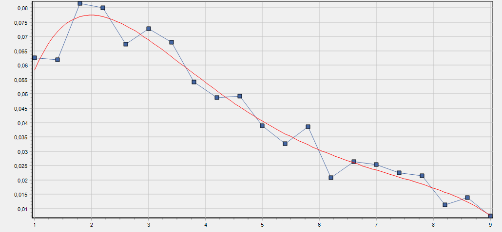
The example demonstrated that vector and matrix expressions can be used together with array and matrix variables and, in some cases, they are more flexible, because their components can depend on other variables.

These new improvements of linear algebra capabilities allowed realizing vector basis for linear least squares approximation. Here is the source code of an approximation example using the vector basis:

var
  approximator: TLinearApproximator;
  basis: TLinearBasis;
  func: string;
  parameters: TArray<TVariable>;
  exponents, cValues: TArray<TFloat>;
  A: TVariable;
  dim, order: integer;
begin
  // Setting parameters for approximation.
  dim:= 1; // One dimension.
  // exponent values
  exponents:= TArray<TFloat&ht;.Create(0.0, 0.5, -0.5, 0.7, -0.7); 
  order:= Length(exponents); // Basis order is the size of the array.
  // Vector variable for exponent array.
  A:= TRealArrayVariable.Create('A', exponents); 
  parameters:= TArray<TVariable>.Create(A); // Parameters for Vector basis.
  func:= 'e^(A*X[0])'; // Vector function for basis - returns real vector.
  
  // Create the basis with the specified function and parameters.
  basis:= TLinearVectorBasis.Create('X', 'C', order, dim, parameters, func);

  approximator:= TLinearLeastSquares.Create; // Linear approximator.
  // Calculate the optimal basis coefficients.
  cValues:= approximator.Approximate(basis, vData, fData); 

  // Using the approximation (basis with optimal coefficients)...
end;

As can be seen from the code, approximation basis function has very compact form – ‘e^(A*X[0])’, because it uses vector variable ‘A’ and so, the return value of the function is real vector. The result of the approximation for some given data is the following:

F(X, C, A) = C•e^(A*X[0])

F(X) = [0.015894261869996 -0.000559709975637631 0.560703382127893
             6.67799570997929E-5 -0.60704298180144]•e^([0 0.5 -0.5 0.7 -0.7]*X[0])

Advantages of using vector basis are:

Simple basis function expression (in vector form).
Easily create high-order basis (using big array parameter).
Use arbitrary coefficients for the basis (fractional exponents, powers and so on).
Change the basis without changing the function (use other values of the parameter array ‘A’).

In addition to the vector and matrix expressions, there are some other symbolic features in the version 2.5. One feature is calculating symbolic expression for n-order or mixed derivative with one function call. The code below calculates mixed derivative of a complicated expression:

var
  translator: TTranslator;
  F, Dxy: string;
begin
  translator:= TTranslator.Create;

  F:= '(y-A*ln(y))/x+B*(v(x+y))^(2/Pi)';
  Dxy:= translator.Derivative(F, TArray<string>.Create('x','y'));

  // using mixed derivative Dxy...
end;

The output result for the derivative is:

F(x,y)  = (y-A*ln(y))/x+B*(v(x+y))^(2/Pi)
dF/dxdy = (-1+A/y)/x^2+B*(1/p-1)*(x+y)^(1/p-2)/p

Note, that after derivative evaluation the result expression simplified. New simplifications in version 2.5 are: put minus operator under sum and product expressions (first expression in the sum ‘(-1+A/y)/x^2’); simplification of square root and power expressions (second expression in the sum ‘B*(1/p-1)*(x+y)^(1/p-2)/p’). Finally, there is new symbolic function that allows getting all variable names from math expressions. Here is an example of using the function:

var
  F: string;
  Names: TArray<string>;
begin
  F:= 'A[i]*sin(2*Pi*x)+A[j]*cos(2*Pi*y)+B[i]*e^((1+I)*x)+B[j]*e^((1-2I)*y)';
  Names:= TTranslator.VariableNames(F);

  // using the Names array...
end;

The result is the following:

F = A[i]*sin(2*Pi*x)+A[j]*cos(2*Pi*y)+B[i]*e^((1+I)*x)+B[j]*e^((1-2I)*y)
Variable names: A, i, x, j, y, B

Note, that the function does not include variable names in the result twice (i, j, x, y, A, B). In addition, standard constants, like Pi and Euler number, not included in the names list.

The version 2.5 is already available here. Source code of the example application can be downloaded from here. Other examples of using vector/matrix operations, expressions and vector basis with graphics visualization included in demo projects of the version 2.5.

Bruno Fierens

This blog post has not received any comments yet.

All Blog Posts | Next Post | Previous Post

Explore All Products

Blog

New linear algebra operations and symbolic features in TMS Analytics & Physics library

Friday, July 13, 2018

This blog post has not received any comments yet.

Add a new comment

Blog Search